In this Technical Tip we discuss the differences between SN/miners rule and fracture mechanics-based techniques for evaluating the fatigue life of components exposed to cyclic stress and highlight the deficiencies of the SN/Miners rule approach.

An SN curve, or Wolher curve, for a particular material in a specific heat treatment condition, is obtained by testing a large number of notched, or unnotched, specimens at specific stress amplitudes until the specimens fail. The stress amplitude and numbers of cycles to failure for each of these tests is then plotted on a log/log graph with stress amplitude (Sa) on the ordinate (Y axis) and the number of cycles to failure N on the abscissa (X axis), Figure 1. In an ideal situation, the material is considered isotropic, continuous and homogeneous, and the stresses in a fatigue test are consistently controlled. It is further assumed that there are no flaws or defects in the material, which, in practice, is almost impossible to achieve and even under ideal lab conditions there is considerable variability in the number of cycles to failure (left image in Figure 1). Such testing produces a band of data representing the fatigue life at various stress levels, which, using statistical methods, can be used to define limits for various levels of risk of failure (right image in Figure 1).

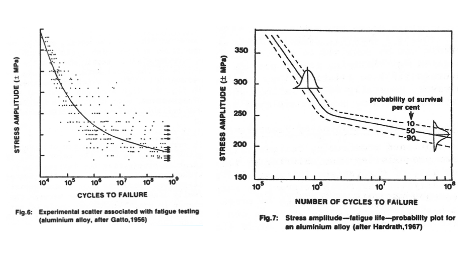
Figure 2: Collage of figures showing typical stress amplitude vs number of cycles to failure material data (shown left) and schematic characterisation thereof (shown right), highlighting i) the significant scatter in typical S/N data (left), and ii) the statistical approach used to address the risk of failure.

At low stress amplitudes, the SN curve of many ferrous materials asymptotes to a fatigue/endurance limit, below which failure by fatigue is unlikely to occur. Such SN curves allow a designer to i) define a stress level which will give an acceptable fatigue life, or ii) to ensure the stress is kept below the endurance limit to prevent fatigue failure. However, it is often overlooked that since this data is developed by constant amplitude testing, S/N curves are strictly only relevant to constant amplitude loading scenarios.

Under variable amplitude loading situations, the cumulative damage hypothesis, or the so-called Palmgren Miner rule, is often employed to adapt SN results developed for constant amplitude loading to variable amplitude loading. Miner’s rule is based on the flawed postulate that i) the application of n_i load cycles with a stress amplitude of S_ai and corresponding fatigue life N_i will consume n_i/N_i% of the component’s fatigue resistance, and ii) when the sum cumulative damage of all the load cycles at different amplitudes, Equation 1, equals one failure will occur.

Equation 1

This hypothesis has no fundamental basis and has been shown by testing carried out by Miner in 1945 that the failure could occur when the Σn/N ranged from 0.61 to 1.45. The rule does not make any allowances for inter alia the loading frequency, the ratio of maximum to minimum stress, the sequence of loading, crack tip plasticity or crack closure effects. Subsequent testing carried out by various researchers, including that undertaken by NASA in 1959 to determine the effect of the load sequence, showed the Σn/N ranged from below 0.6 to more than 4. Even given these inadequacies, this approach is still employed today.

While SN (Stress versus Number of cycles to failure) is a viable and useful model for predicting constant amplitude fatigue life during the design phases, it excludes many real-life factors encountered in practice. Materials contain imperfections, and particularly in welded fabrications, the material is locally variable, in terms of its micro-structure, mechanical properties and fracture toughness. It may also contain residual stresses, which in welded components often approach yield stress magnitude, unless a suitable post-weld heat treatment is consistently and correctly employed. Additionally, when information regarding prior component history, machinery operating conditions, and the possible presence of hidden flaws or defects is not readily available, the SN approach becomes even less reliable.

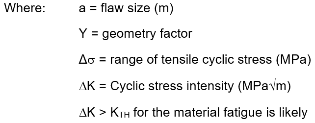
From a fracture mechanics fatigue perspective, fatigue cracks initiate and propagate when the magnitude of the local cyclic stress intensity, defined in previous Tech Tips and by Equation 2, in a material exceeds the threshold value for that particular material/environment. This typically occurs in areas of stress concentration, which occur in the vicinity of flaws or where there are abrupt changes in section, such as fillet radii and threads. As the crack grows, ‘a’, and hence ΔK, increases and when the maximum stress intensity exceeds the fracture toughness of the material (i.e. K>K_IC), failure occurs by fast overload fracture mechanisms.

Equation 2

Once a crack has initiated, crack growth is characterised by the Paris Equation, Equation 3, which defines the mid-section of the graph and relates the rate of crack growth da/dN to the cyclic stress intensity amplitude (ΔK).

Equation 3

As shown in Figure 2 and Figure 3, when ΔK is sufficiently small, i.e. below a so-called ‘threshold’ value, ΔK_TH, fatigue crack initiation will not occur. It should be noted that, although the no crack growth assumption is applicable in terms of continuum mechanics, it does not mean that no damage occurs at the sub-grain size level.